Understanding Fastai's fit_one_cycle method

February 19, 2019, 7 min read

TL;DR: fit_one_cycle() uses large, cyclical learning rates to train models significantly quicker and with higher accuracy.

When training Deep Learning models with Fastai it is recommended to use the fit_one_cycle() method, due to its better performance in speed and accuracy, over the fit() method. In short, fit_one_cycle() is Fastai’s implementation of Leslie Smith’s 1cycle policy. Smith developed, refined and publicised his methodology over three research papers:

In this article we’ll explore the underlying concepts behind the 1cycle policy and try to understand why this method works better.

The problem with Learning Rate

Training a Deep Neural Network (DNN) is a difficult global optimization problem. Learning Rate (LR) is a crucial hyper-parameter to tune when training DNNs. A very small learning rate can lead to very slow training, while a very large learning rate can hinder convergence as the loss function fluctuates around the minimum, or even diverges.

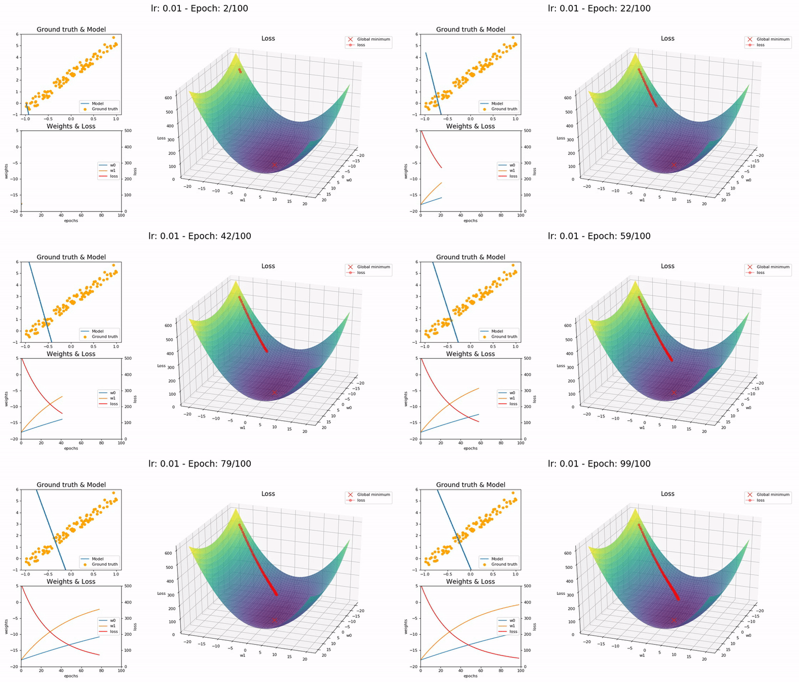
Too small LR (0.01). The model fails to converge within 100 epochs. More epochs—and time—required:

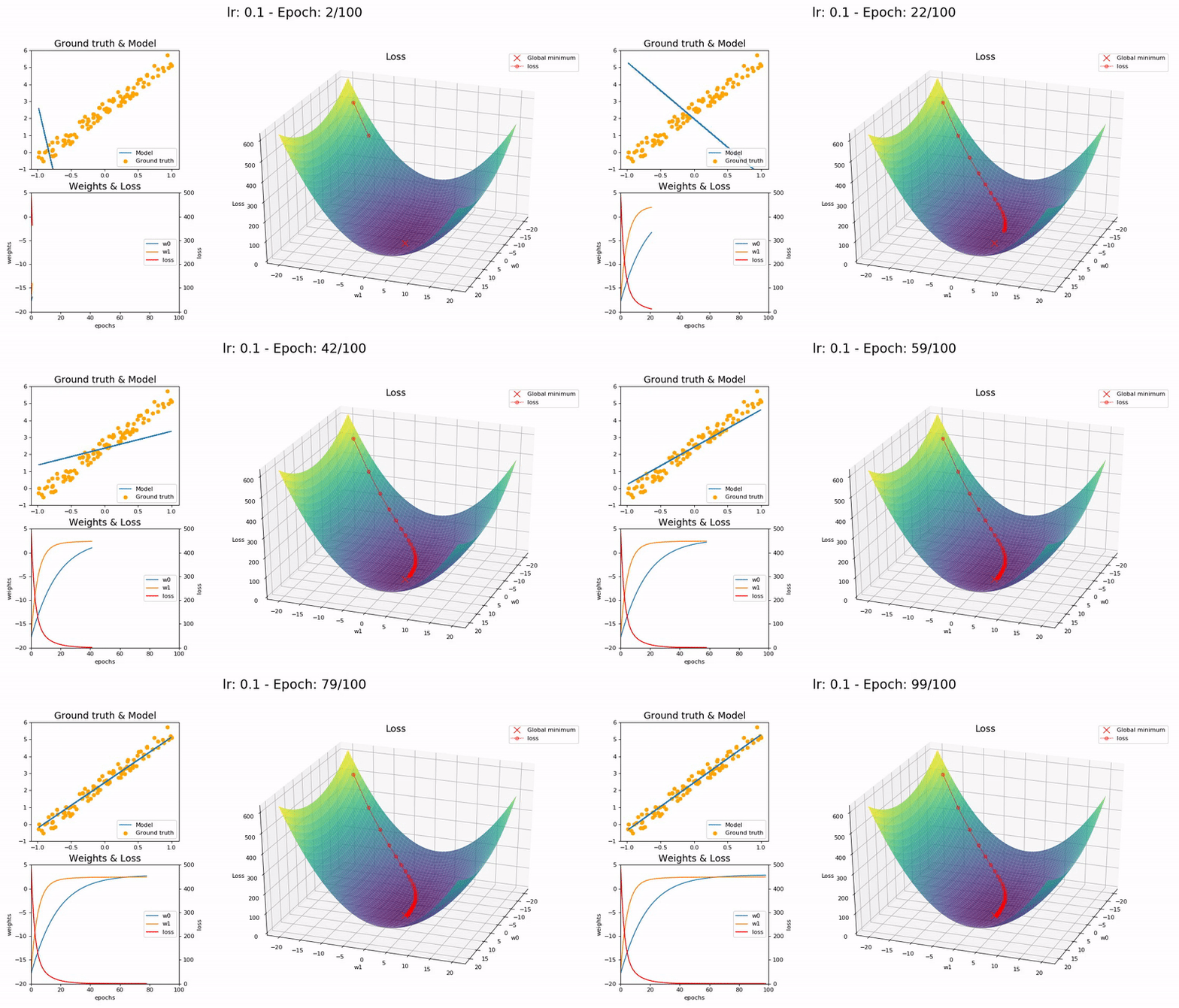
Good LR (0.1). The model converges successfully within 100 epochs:

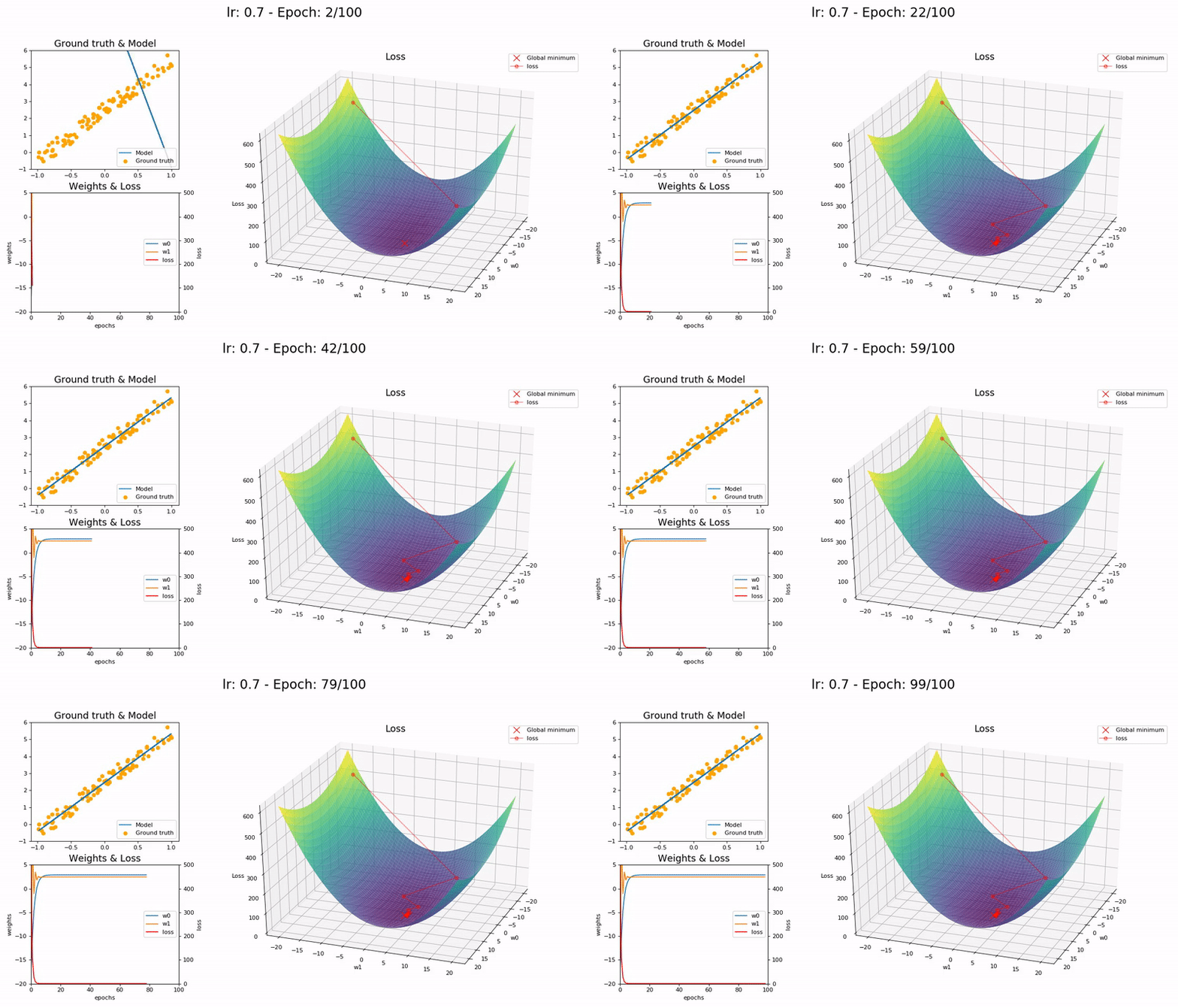
Optimal LR (0.7). The model converges successfully, very quickly, in under 10 epochs:

Large LR (0.99). The model fails to converge as the loss function fluctuates around the minimum:

Too large LR (1.01). The model diverges quickly:

(Graphs by José Fernández Portal)

A low learning rate is slow but more accurate. As learning rate increases so does the training speed, until learning rate gets too large and diverges. Finding the sweet spot requires experimentation and patience. An automated way of calculating the optimal learning rate is to perform a grid search, but this is a time consuming process.

In practice, learning rate is not static but changes as training progresses. It is desirable to start with an optimal learning rate (for speed) and gradually decrease it towards the end (for accuracy). There are two ways to achieve this: learning rate schedules and adaptive learning rate methods.

Learning rate schedules are mathematical formulas that decrease the learning rate using a particular strategy (Time-Based Decay, Step Decay, Exponential Decay, etc). That strategy/schedule is set before training commences and remains constant throughout the training process. Thus, learning rate schedules are unable to adapt to the particular characteristics of a dataset. Adaptive learning rate methods (Adagrad, Adadelta, RMSprop, Adam, etc) alleviate that problem but are computationally expensive. See ”An overview of gradient descent optimization algorithms” (Ruder, 2016) for an in-depth analysis.

Cyclical Learning Rates

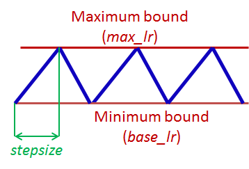
Smith discovered a new method for setting learning rate, named Cyclical Learning Rates (CLRs). Instead of using a fixed, or a decreasing learning rate, the CLR method allows learning rate to continuously oscillate between reasonable minimum and maximum bounds.

One CLR cycle consists of two steps; one in which the learning rate increases and one in which it decreases. Each step has a size (called stepsize), which is the number of iterations (e.g. 1k, 5k, etc) where learning rate increases or decreases. Two steps form a cycle. Concretely, a CLR cycle with stepsize of 5,000 will consist of 5,000 + 5,000 = 10,000 total iterations. A CLR policy might consist of multiple cycles.

CLRs are not computationally expensive and eliminate the need to find the best learning rate value—the optimal learning rate will fall somewhere between the minimum and maximum bounds. A cyclical learning rate produces better overall results, despite the fact that it might hinder the network performance temporarily.

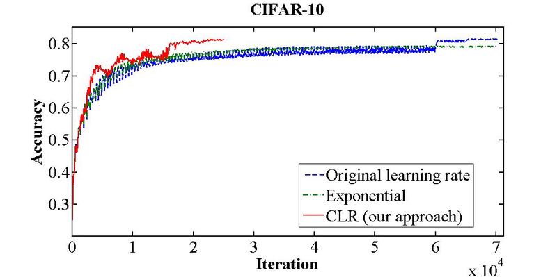
The above figure shows the training accuracy of the CIFAR-10 dataset over 70,000 iterations. A fixed learning learning rate (blue line) achieves 81.4% accuracy after 70,000 iterations, while the CLR method (red line) achieves the same within 25,000 iterations.

“The essence of this learning rate policy comes from the observation that increasing the learning rate might have a short term negative effect and yet achieve a longer term beneficial effect.” Smith

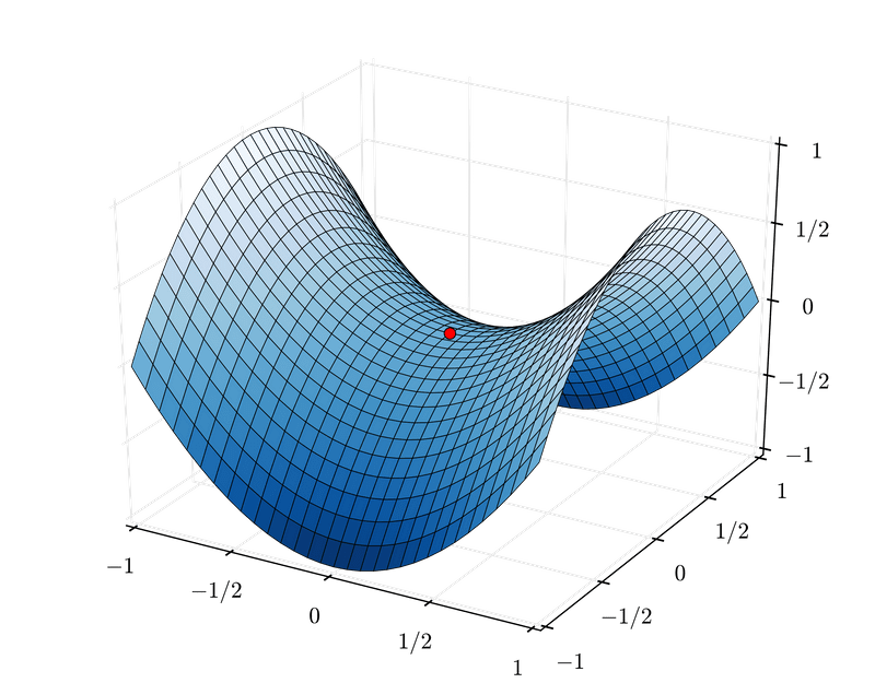
Cyclical Learning Rates are effective because they can successfully negotiate saddle points, which typically have small gradients (flat surfaces) and can slow down training when learning rate is small. The best way to overcome such obstacles is to speed up and to move fast until a curved surface is found. The increasing learning rate of CLRs does just that, efficiently.

Learning Rate range test

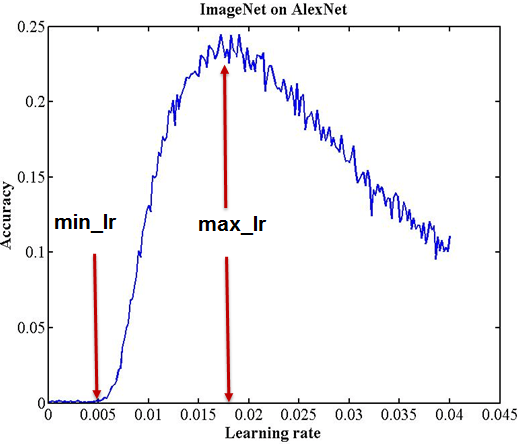
Smith also devised a simple method for estimating reasonable minimum and maximum learning rate bounds; the LR range test. The test involves running a model for several epochs, where learning rate starts at a low value and increases linearly towards a high value. A plot of accuracy versus learning rate shows when accuracy starts to increase and when it slows down, becomes ragged, or declines. The following LR range test plot shows two points that are good candidates for the minimum and maximum bounds:

Subsequently, a Cyclical Learning Rate policy that varies between these bounds will produce good classification results, often with fewer iterations and without any significant computational expense, for a range of architectures.

Super-convergence and 1cycle policy

Building on his CLR research, Smith followed up with his paper on super-convergence, a phenomenon where neural networks can be trained an order of magnitude faster than with standard training methods.

Super-convergence uses the CLR method, but with just one cycle—which contains two learning rate steps, one increasing and one decreasing—and a large maximum learning rate bound. The cycle’s size must be smaller than the total number of iterations/epochs. After the cycle is complete, the learning rate should decrease even further for the remaining iterations/epochs, several orders of magnitude less than its initial value. Smith named this the 1cycle policy.

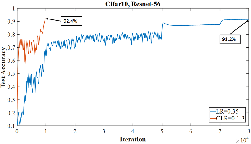
Concretely, in super-convergence, learning rate starts at a low value, increases to a very large value and then decreases to a value much lower than its initial one. The effect of that learning rate movement is a very distinctive training accuracy curve. Traditional training accuracy curves increase, then plateau as the value of learning rate changes (see blue curve, below). Super-convergence training accuracy curves (see red curve, below) have a dramatic initial jump (moving fast as learning rate increases), oscillate or even decline for a bit (while learning rate is very large) and then jump up again to a distinctive accuracy peak (as learning rate decreases to a very small value).

lr vs clr resnet56 — Example of super-convergence training accuracy curve

Smith found that a large learning rate acts as a regularisation method. Hence, when using the 1cycle policy, other regularisation methods (batch size, momentum, weight decay, etc) must be reduced.

How Fastai implements the 1cycle policy

Fastai abstracts all the implementation details of the 1cycle policy and provides an intuitive interface in the form of fit_one_cycle(). The latter calls fit() internally, appending an OneCycleScheduler callback:

  def fit_one_cycle(learn:Learner, cyc_len:int,
    max_lr:Union[Floats,slice]=defaults.lr, moms:Tuple[float,float]=(0.95,0.85),
    div_factor:float=25., pct_start:float=0.3, wd:float=None,
    callbacks:Optional[CallbackList]=None, tot_epochs:int=None,
    start_epoch:int=1)->None:
    "Fit a model following the 1cycle policy."

    max_lr = learn.lr_range(max_lr)
    callbacks = listify(callbacks)
    callbacks.append(OneCycleScheduler(learn, max_lr, moms=moms,
      div_factor=div_factor, pct_start=pct_start,
      tot_epochs=tot_epochs,start_epoch=start_epoch))

    learn.fit(cyc_len, max_lr, wd=wd, callbacks=callbacks)

Calling fit_one_cycle() with only a few basic parameters allows us to reap the benefits of the 1cycle policy with very little effort.